Healthcare Data Quality Example • autoFlagR

Introduction

This vignette demonstrates using autoFlagR for data quality auditing in a healthcare context. We’ll work through a complete example using simulated Electronic Health Records (EHR) data.

Load Required Packages

library(autoFlagR)
library(dplyr)
#> 
#> Attaching package: 'dplyr'
#> The following objects are masked from 'package:stats':
#> 
#>     filter, lag
#> The following objects are masked from 'package:base':
#> 
#>     intersect, setdiff, setequal, union
library(ggplot2)

Create Example Healthcare Dataset

set.seed(123)

# Simulate healthcare data
n_patients <- 500
healthcare_data <- data.frame(
  patient_id = 1:n_patients,
  age = round(rnorm(n_patients, 55, 15)),
  systolic_bp = round(rnorm(n_patients, 120, 15)),
  diastolic_bp = round(rnorm(n_patients, 80, 10)),
  cholesterol = round(rnorm(n_patients, 200, 40)),
  glucose = round(rnorm(n_patients, 100, 20)),
  bmi = round(rnorm(n_patients, 28, 5), 1),
  gender = sample(c("Male", "Female"), n_patients, replace = TRUE),
  diagnosis = sample(c("Hypertension", "Diabetes", "Normal"), n_patients, replace = TRUE, prob = c(0.3, 0.2, 0.5))
)

# Introduce known anomalies
healthcare_data$age[1:10] <- c(250, 180, 200, 190, 185, 175, 170, 165, 160, 155)  # Impossible ages
healthcare_data$systolic_bp[11:15] <- c(300, 280, 290, 275, 285)  # Extreme blood pressure
healthcare_data$cholesterol[16:20] <- c(600, 580, 590, 570, 585)  # Very high cholesterol
healthcare_data$glucose[21:25] <- c(5, 3, 4, 2, 6)  # Unrealistically low glucose

# Create ground truth labels and add to data
healthcare_data$is_anomaly_truth <- rep(FALSE, n_patients)
healthcare_data$is_anomaly_truth[1:25] <- TRUE  # First 25 are anomalies

head(healthcare_data)
#>   patient_id age systolic_bp diastolic_bp cholesterol glucose  bmi gender
#> 1          1 250         111           70         167      90 24.6   Male
#> 2          2 180         105           70         188     105 30.9 Female
#> 3          3 200         135           80         164      89 24.5 Female
#> 4          4 190         131           79         225     124 25.3 Female
#> 5          5 185          97           55         245     103 31.9 Female
#> 6          6 175         119           90         285      88 25.6 Female
#>      diagnosis is_anomaly_truth
#> 1 Hypertension             TRUE
#> 2     Diabetes             TRUE
#> 3       Normal             TRUE
#> 4       Normal             TRUE
#> 5 Hypertension             TRUE
#> 6       Normal             TRUE

Preprocess Data

# Prepare data for anomaly detection
prepared <- prep_for_anomaly(
  healthcare_data,
  id_cols = "patient_id",
  scale_method = "mad"
)

# View preprocessing metadata
str(attr(prepared, "metadata"))
#>  NULL

Score Anomalies

# Score anomalies using Isolation Forest
scored_data <- score_anomaly(
  healthcare_data,
  method = "iforest",
  contamination = 0.05,
  ground_truth_col = "is_anomaly_truth",
  id_cols = "patient_id"
)

# View summary statistics
summary(scored_data$anomaly_score)
#>    Min. 1st Qu.  Median    Mean 3rd Qu.    Max. 
#>  0.0000  0.5975  0.7217  0.6988  0.8340  1.0000

Flag Top Anomalies

# Flag top anomalies
flagged_data <- flag_top_anomalies(
  scored_data,
  contamination = 0.05
)

# Count anomalies
cat("Total anomalies flagged:", sum(flagged_data$is_anomaly), "\n")
#> Total anomalies flagged: 25
cat("Anomaly rate:", mean(flagged_data$is_anomaly) * 100, "%\n")
#> Anomaly rate: 5 %

Visualize Results

# Plot anomaly score distribution
ggplot(flagged_data, aes(x = anomaly_score)) +
  geom_histogram(bins = 50, fill = "steelblue", alpha = 0.7, color = "black") +
  geom_vline(xintercept = attr(flagged_data, "anomaly_threshold"),
             color = "red", linetype = "dashed", linewidth = 1) +
  labs(
    title = "Distribution of Anomaly Scores",
    x = "Anomaly Score",
    y = "Frequency"
  ) +
  theme_minimal()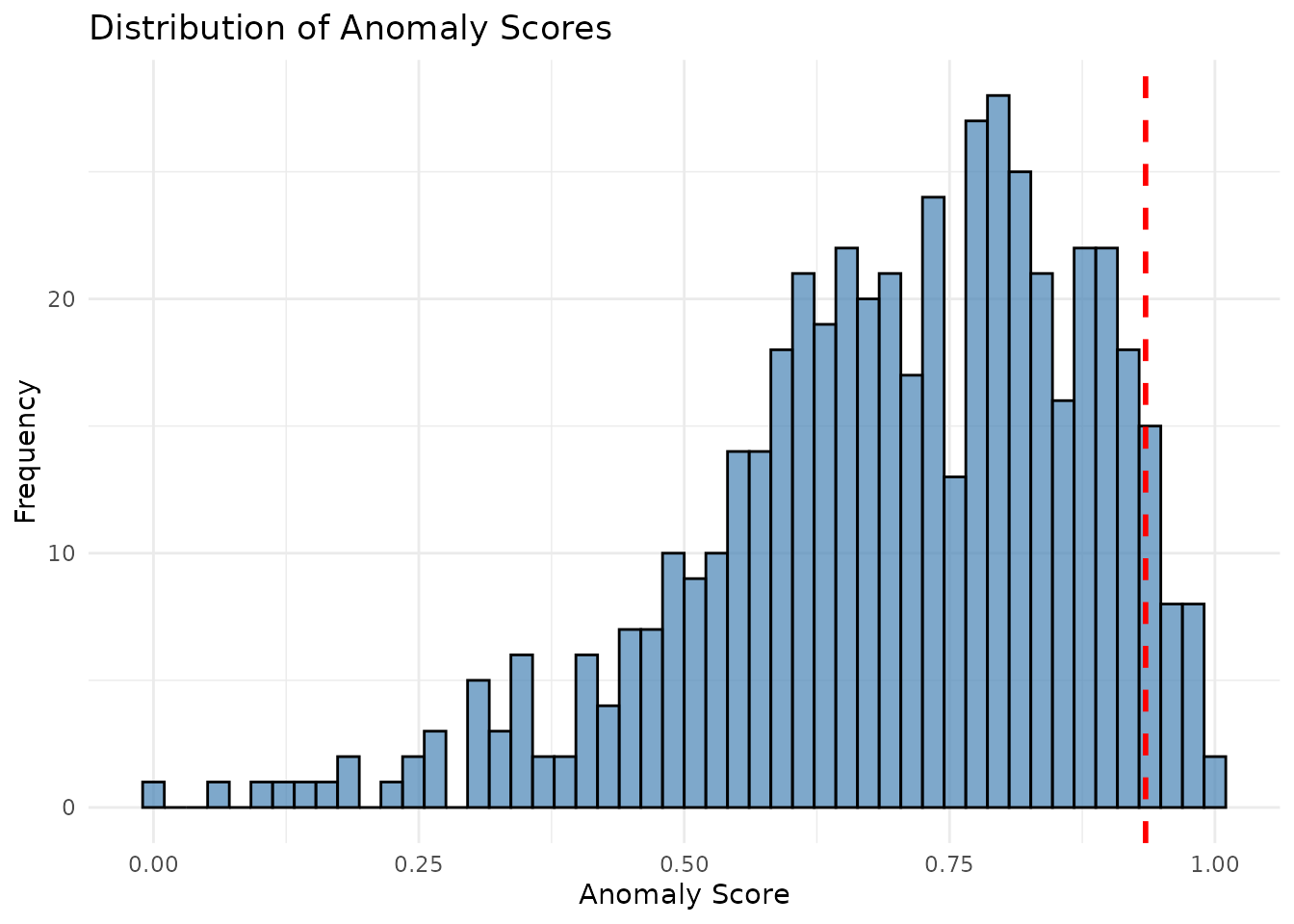

Extract Top Anomalies

# Get top 10 anomalies
top_anomalies <- get_top_anomalies(flagged_data, n = 10)

# View top anomalies
top_anomalies[, c("patient_id", "age", "systolic_bp", "cholesterol", 
                  "glucose", "anomaly_score", "is_anomaly")]
#>    patient_id age systolic_bp cholesterol glucose anomaly_score is_anomaly
#> 1         299  55         123         218      87     1.0000000       TRUE
#> 2          60  58         111         221     105     0.9914128       TRUE
#> 3         445  45         113         217     116     0.9844411       TRUE
#> 4         239  60         119         191     104     0.9831260       TRUE
#> 5         362  65         122         186     116     0.9786138       TRUE
#> 6          82  61         118         234      78     0.9771008       TRUE
#> 7         469  56         119         169     117     0.9769758       TRUE
#> 8          48  48         130         225     100     0.9762012       TRUE
#> 9          51  59         133         199      96     0.9747442       TRUE
#> 10        252  47         118         235      98     0.9721997       TRUE

Benchmarking (if ground truth available)

# Extract benchmark metrics
if (!is.null(attr(scored_data, "benchmark_metrics"))) {
  metrics <- extract_benchmark_metrics(scored_data)
  
  cat("AUC-ROC:", metrics$auc_roc, "\n")
  cat("AUC-PR:", metrics$auc_pr, "\n")
  cat("Top-10 Recall:", metrics$top_k_recall$top_10, "\n")
  cat("Top-50 Recall:", metrics$top_k_recall$top_50, "\n")
}
#> AUC-ROC: 0.9796211 
#> AUC-PR: 0.0256281 
#> Top-10 Recall: 0 
#> Top-50 Recall: 0

Generate Comprehensive Report

# Generate PDF audit report (saves to tempdir() by default)
generate_audit_report(
  healthcare_data,
  filename = "healthcare_audit_report",
  output_dir = tempdir(),
  output_format = "pdf",
  method = "iforest",
  contamination = 0.05,
  ground_truth_col = "is_anomaly_truth",
  id_cols = "patient_id"
)

The report will include: - Executive summary with key metrics - Anomaly score distribution - Prioritized audit listing (heatmap) - Bivariate visualizations - Distribution comparisons - Benchmarking results (if ground truth provided)

Summary

This example demonstrated: 1. Creating and preprocessing healthcare data 2. Scoring anomalies using Isolation Forest 3. Flagging top anomalies for review 4. Visualizing results 5. Extracting benchmark metrics 6. Generating professional audit reports

For more details, see the Function Reference.